Screen Recording

by Craig Hutton

Demonstrating the functionality of a given function or technique is often more effective and efficient when using animated GIFs. The following two software will help you create GIFs with ease and for free!

• screentogif.com - Windows
• getkap.co - Mac

High Precision Summations

by Matthew Parker

Log space is used for higher precision

dpois(x = 5, lambda = 1000) # sample from a Poisson Distribution

## [1] 0

dpois(x = 5, lambda = 1000, log=T)

## [1] -970.2487

This is good for multiplication: \(\log(a\times b) = \log(a) + \log(b)\)

dpois(x = 5, lambda = 1000)^2

## [1] 0

2*dpois(x = 5, lambda = 1000, log=T)

## [1] -1940.497

But it fails for addition: \(\log(a+b)=?\)

For example, if we want to calculate \(a + b\), but only have accurate \(\log(a)\) and \(\log(b)\):

\[a + b = \exp(\log(a)) + \exp(\log(b))\]

In this case, exponentiation destroys precision!

dpois(x = 5, lambda = 1000, log=T)

## [1] -970.2487

exp(dpois(x = 5, lambda = 1000, log=T))

## [1] 0

So how can we calculate:

dpois(x = 5, lambda = 1000) + dpois(x = 5, lambda = 1000)

## [1] 0

Solution: keep the largest part in log space!

suppose \(a \geq b\):

\[ \begin{aligned} \log(a + b) &= \log(\exp(\log(a)) + \exp(\log(b))) \\ &= \log( \exp(\log(a)) \times (1+\exp(\log(b)-\log(a))) ) \\ &= \log( \exp(\log(a)) ) + \log( 1+\exp(\log(b)-\log(a))) ) \\ &= \log(a) + \text{log1p}( \exp(\log(b)-\log(a)) ) \end{aligned} \]

Let’s define the function to accomplish this task

logSumExp <- function(x) {
  if(all(is.infinite(x))) { return(x[1]) }
  x = x[which(is.finite(x))]
  ans = x[1]
  for(i in seq_along(x)[-1]) {
    ma = max(ans,x[i])
    mi = min(ans,x[i])
    ans = ma + log1p(exp(mi-ma))
  }
  return(ans)
}

and demonstrate its use:

x = c(dpois(x = 5, lambda = 1000, log = T), 
      dpois(x = 5, lambda = 1000, log = T))
logSumExp(x)

## [1] -969.5556

Voila, the precision is preserved!

Axis labels

by Andriy Koval

library(magrittr)
library(dplyr)
library(ggplot2)
library(lemon)

When faceting a plot, we may need to place axis labels on each facet (especially if we have many of them):

mtcars %>% 
  ggplot(aes(x=disp, y = mpg))+
  geom_point()+
  facet_wrap(~cyl, ncol=1)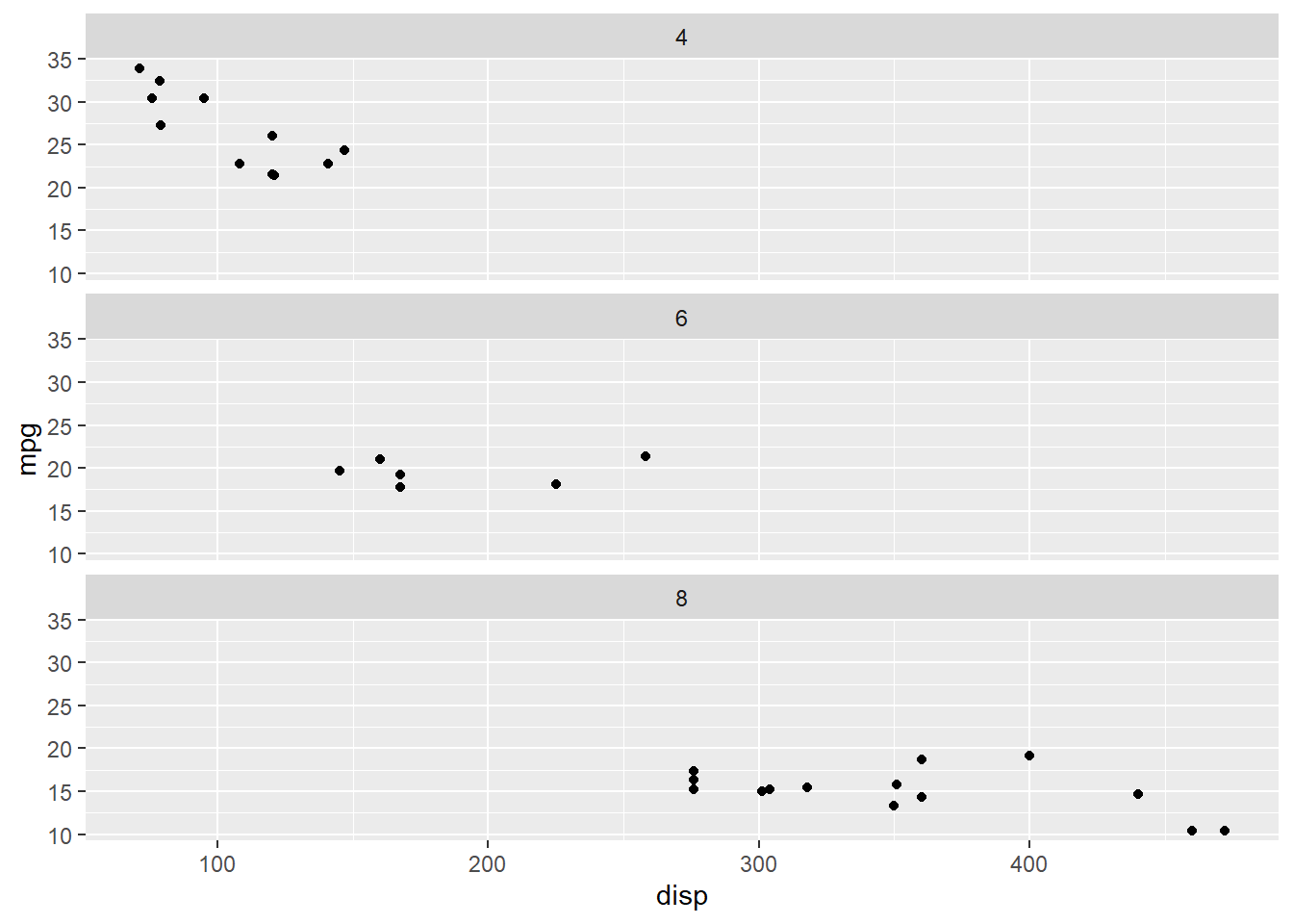

One way of achieving this is to use scale = "free_x" argument, but if data on the faceted levels covers different ranges of values, the limits of the scale will be adjusted:

mtcars %>% 
  ggplot(aes(x=disp, y = mpg))+
  geom_point()+
  # facet_wrap(~cyl, ncol=1) 
  facet_wrap(~cyl, ncol=1, scales = "free_x") # puts tick marks, but distorts scale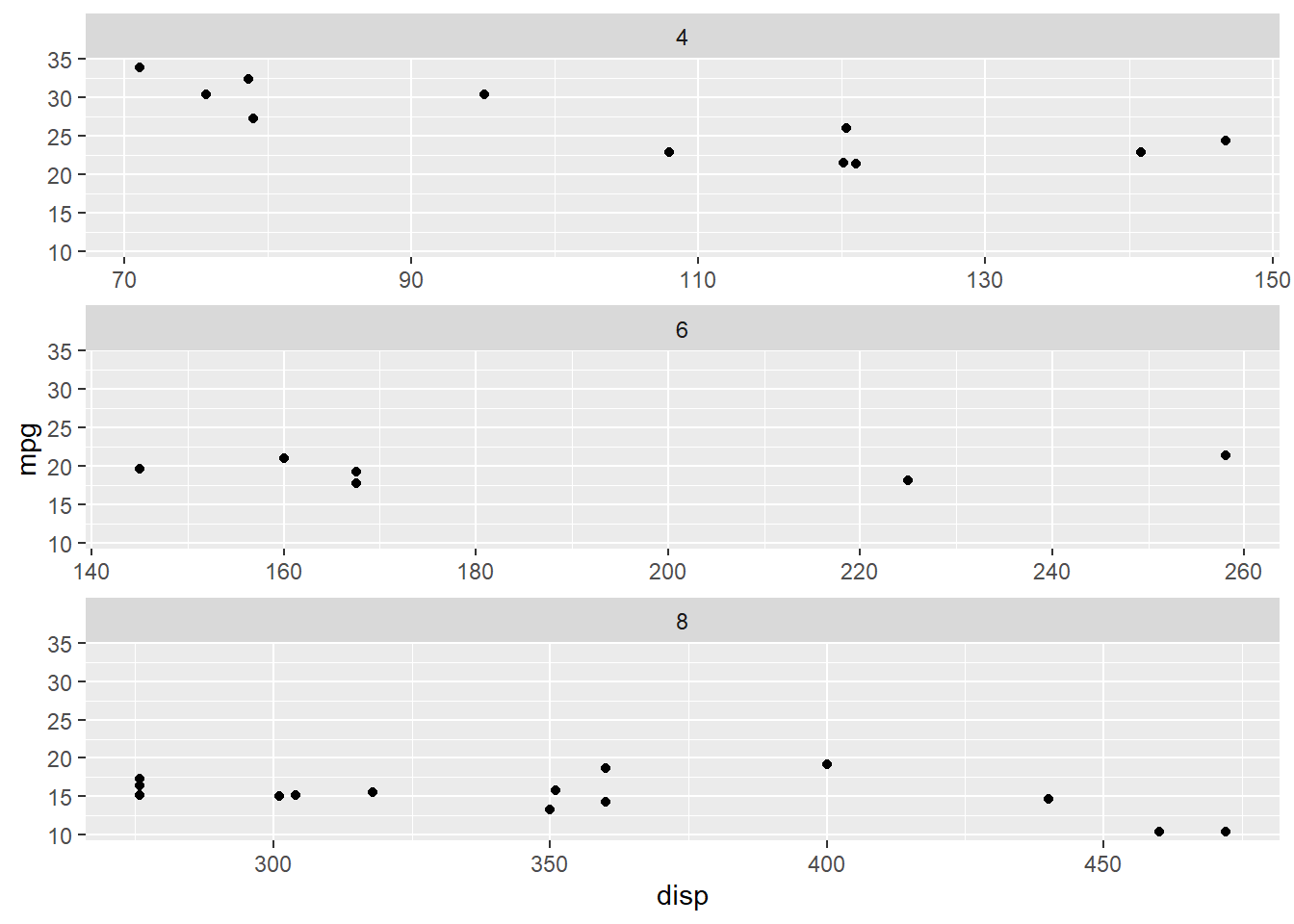

Comes in the lemon package, which provides functions facet_rep_wrap() and facet_rep_grid() to offer exactly this flexibility. You can also use the arguments you normally pass to facet_wrap() or facet_grid(), respectively:

mtcars %>% 
  ggplot(aes(x=disp, y = mpg))+
  geom_point()+
  # facet_wrap(~cyl, ncol=1) 
  # facet_wrap(~cyl, ncol=1, scales = "free_x") # puts tickmarks, but distorts scale
  lemon::facet_rep_wrap(~cyl,ncol=1, repeat.tick.labels = TRUE)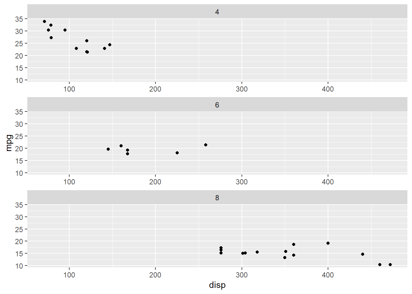

Tidy Evals

by Kyle Belanger

library(magrittr)
library(dplyr)
library(ggplot2)
library(lemon)

When turning your ggplots into functions, we can use aes_string function to pass quoted strings as variable names:

make_faceted_scatter <- function(d,xvar,yvar){
  mtcars %>% 
    ggplot(aes_string(x=xvar, y = yvar))+
    geom_point()
}
mtcars %>% make_faceted_scatter("disp","mpg")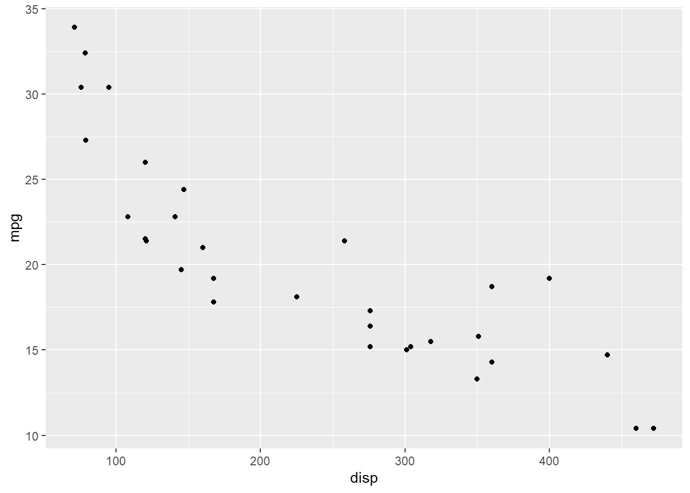

However, passing an unquoted variable names to function required resorting to rlang package to translate bares (unquoted names) to quosures in functions:

Unfortunately, this did not play well with facets. However, since 0.4.0 version, rlang provides a shortcut for this implementation using {{}}, which pairs up with the new (ggplot2 3.0.0) helper function vars() in facet_wrap() to make it work:

make_faceted_scatter <- function(d,xvar, yvar,fvar){
  mtcars %>% 
    ggplot(aes(x={{xvar}}, y = {{yvar}}))+
    geom_point()+
    lemon::facet_rep_wrap(vars({{fvar}}),ncol=1, repeat.tick.labels = TRUE)
}
mtcars %>% make_faceted_scatter(disp,mpg,cyl)

Auto-referening in plots

by Kyle Belanger

library(magrittr)
library(dplyr)
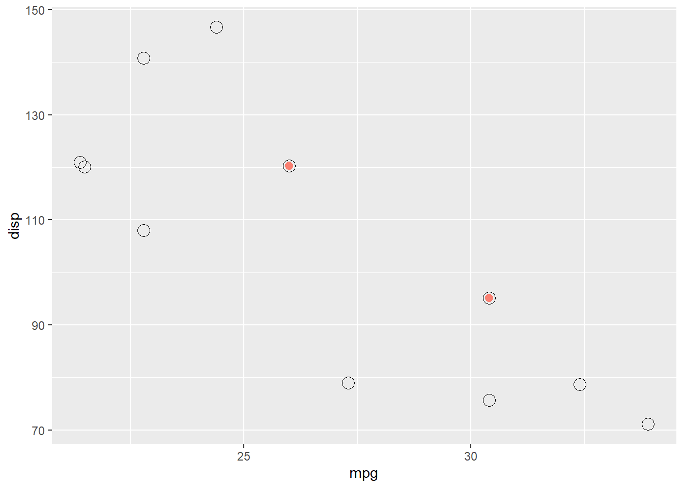
library(ggplot2)

When building ggplot2 objects we might need to build a layer that uses only a subset of the sourced data. For example, in a scatterplot of mpg and disp among 4-cylinder cars

mtcars %>% 
  filter(cyl == 4) %>%
    ggplot(aes(x = mpg, y = disp ))+
      geom_point(shape = 1,  size =4)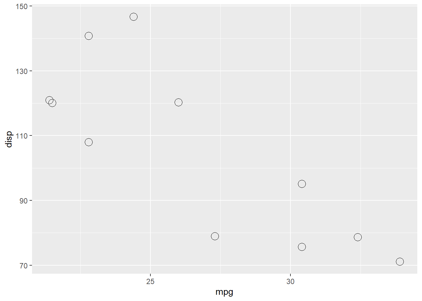

we may want to highlight only those with 5 gears. This could be accomplished by passing data = to the extra geom that would draw the highlight:

mtcars %>% 
  filter(cyl == 4) %>%
    ggplot(aes(x = mpg, y = disp ))+
      geom_point(shape = 1,  size =4)+
      geom_point(shape = 20, size = 4,data = mtcars %>% filter(cyl==4, gear == 5))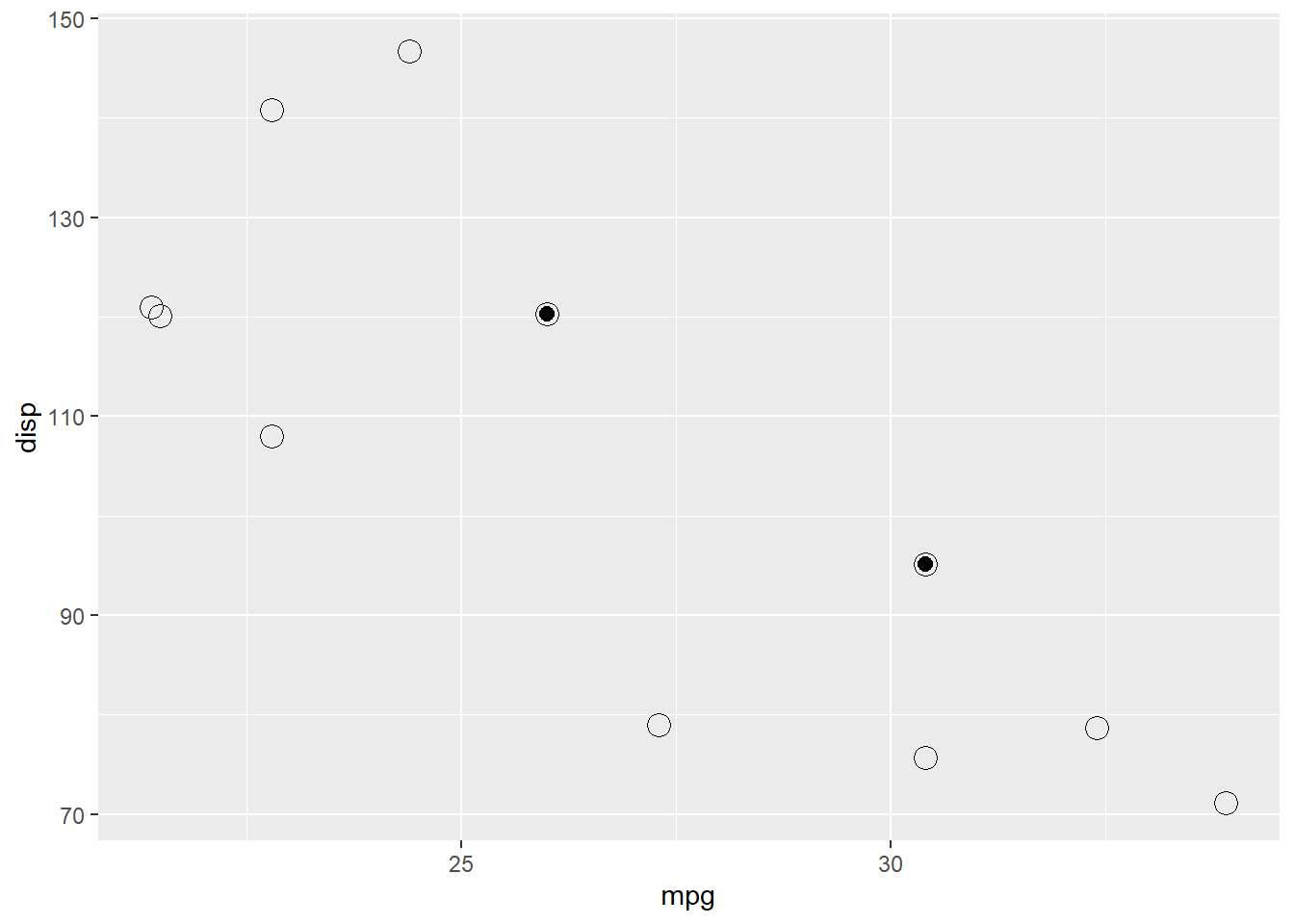

This approach, however, has a major disadvantage: you have to repeat the transformations (in this case only filter) that take place between the source data and the ggplot2 canvas. ggplot2 3.0.0 offers a more elegant solution by surrounding the ggplot canvas in {} and using . placeholder to refer to the data set that was passed to aes():

mtcars %>% 
  filter(cyl == 4) %>%
  {# ! notice !
    ggplot(.,aes(x = mpg, y = disp ))+
      geom_point(shape = 1, size = 4)+
      geom_point(shape = 20, size = 4,color = "salmon", data = . %>% filter(gear == 5))
  }# ! notice !